Documentation
For full documentation, please refer to the following paper:
The Oxford Radar RobotCar Dataset: A Radar Extension to the Oxford RobotCar Dataset
Dan Barnes, Matthew Gadd, Paul Murcutt, Paul Newman and Ingmar Posner
[Paper]
@inproceedings{RadarRobotCarDatasetICRA2020,
  address = {Paris},
  author = {Dan Barnes and Matthew Gadd and Paul Murcutt and Paul Newman and Ingmar Posner},
  title = {The Oxford Radar RobotCar Dataset: A Radar Extension to the Oxford RobotCar Dataset},
  booktitle = {Proceedings of the IEEE International Conference on Robotics and Automation (ICRA)},
  url = {https://arxiv.org/abs/1909.01300},
  pdf = {https://arxiv.org/pdf/1909.01300.pdf},
  year = {2020}
}
For additional documentation on the RobotCar platform and sensor data apart from the Navtech Radar, Velodyne LIDAR and ground
truth radar odometry, please refer to the original Oxford RobotCar Dataset 1, details of which
can be found at:
[Website]
[Documentation]
[Paper]
Dataset Description
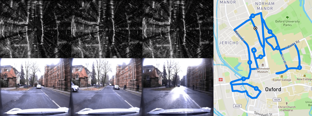
Here we introduce the Oxford Radar RobotCar Dataset, a radar extension to the Oxford RobotCar Dataset, providing
Millimetre-Wave FMCW scanning radar data and optimised ground truth radar odometry for 280 km of driving around
Oxford, UK in January 2019.
We follow the original Oxford RobotCar Dataset route and collect 32 traversals in different traffic, weather and
lighting conditions. Two partial traversals are included which do not cover the entire route.
Modern and increasingly autonomous robots now need to see further, through fog, rain and snow, despite lens flare or when directly facing the sun. Millimetre-Wave radar is capable of of consistent sensor observations in such conditions where other sensor modalities such as vision and LIDAR may fail.
Our radar is a Navtech CTS350-X Frequency-Modulated Continuous-Wave (FMCW) scanning radar and in the configuration used provides 4.38 cm in range resolution and 0.9 degrees in rotation resolution with a range up to 163 m all whilst providing robustness to weather conditions that may trouble other sensor modalities. In other configurations, the Navtech CTS350-X can provide in excess of 650 m in range and higher rotation speeds. However for urban environments the increased resolution was more desirable.
Sensor Suite
We collect data from all the original Oxford RobotCar Dataset sensors excluding the LD-RMS:
- Cameras:
- 1 x Point Grey Bumblebee XB3
- 3 x Point Grey Grasshopper2
- LIDAR:
- 2 x SICK LMS-151 2D LIDAR
- GPS/INS:
- 1 x NovAtel SPAN-CPT ALIGN inertial and GPS navigation system
As well as additionally collecting:
- Radar:
- 1 x Navtech CTS350-X - Mounted in the centre of the roof aligned with the vehicles axes.
- LIDAR
- 2 x Velodyne HDL-32E - Mounted to the left and right of the Navtech CTS350-X radar.
Sensor Locations
The image below shows the location and orientation of each sensor on the vehicle. Precise extrinsic calibrations for each sensor are included in the development tools.
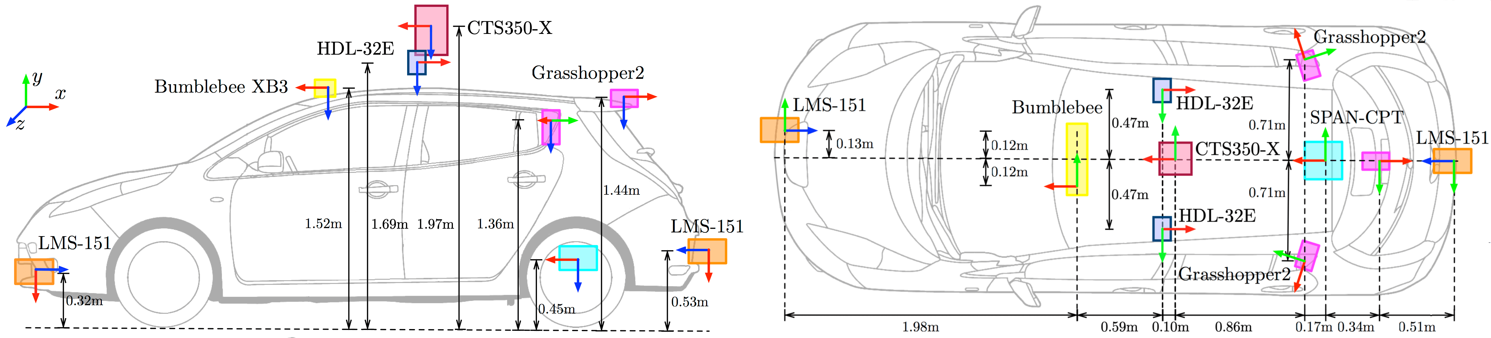
Coordinate frames use the convention x = forward (red), y = right (green), z = down (blue).
Data Format
Unlike the original Oxford RobotCar Dataset we do not chunk sensor data into smaller files. Therefore each download corresponds to one dataset traversal and one sensor (or processed sensor output such as stereo visual odometry).
Using the download script you can download the dataset and easily filtering by dataset and / or sensor. If you would rather download the data manually you can simply follow the links from the individual datasets pages (once your Google account has been authorised for download). Until then you are welcome to try some of the data from the sample datasets (also accessible with the download script).
oxford-radar-robotcar-dataset
├── yyyy-mm-dd-HH-MM-SS-radar-oxford-10k or yyyy-mm-dd-HH-MM-SS-radar-oxford-10k-partial
│   ├── gt
│   │   └── radar_odometry.csv  # ground truth SE2 radar odometry
│   ├── radar
│   │   ├── <timestamp>.png     # Navtech radar data
│   │   ├── ...
│   ├── velodyne_left
│   │   ├── <timestamp>.bin     # Velodyne binary sensor data
│   │   ├── <timestamp>.png     # Velodyne raw sensor data
│   │   ├── ...
│   ├── velodyne_right
│   │   ├── <timestamp>.bin     # Velodyne binary sensor data
│   │   ├── <timestamp>.png     # Velodyne raw sensor data
│   │   ├── ...
│   ├── radar.timestamps
│   ├── velodyne_left.timestamps
│   ├── velodyne_right.timestamps
│   │   # Plus the same layout of files from the original Oxford RobotCar Dataset
│   ├── gps                     # NovAtel gps / ins data
│   │   ├── gps.csv
│   │   └── ins.csv
│   ├── lms_front               # front SICK 2D lidar
│   │   ├── ...
│   ├── lms_rear                # rear SICK 2D lidar
│   │   ├── ...
│   ├── mono_left               # left Grasshopper2 monocular camera
│   │   ├── ...
│   ├── mono_right              # right Grasshopper2 monocular camera
│   │   ├── ...
│   ├── mono_rear               # rear Grasshopper2 monocular camera
│   │   ├── ...
│   ├── stereo                  # front Bumblebee XB3 stereo camera
│   │   ├── ...
│   ├── vo                      # processed visual odometry
│   ├── └── vo.csv
│   ├── lms_front.timestamps
│   ├── lms_rear.timestamps
│   ├── mono_left.timestamps
│   ├── mono_right.timestamps
│   ├── mono_rear.timestamps
│   ├── stereo.timestamps
├── ...
It is intended that all zip archives are extracted into the same directory: this will preserve the folder structure indicated above when multiple traversals and / or sensors are downloaded. The timestamps files contain ASCII formatted data, with each line corresponding to the UNIX timestamp and chunk ID of a single image, LIDAR or radar scan. As mentioned above, in this release we do not chunk the data and so the chunk ID is always set to 1 (included to be consistent with the original Oxford RobotCar Dataset release).
Radar
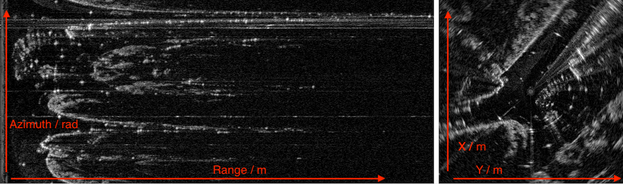
Radar data is released as lossless PNG files in polar form with each row representing the sensor reading at each
azimuth and each column representing the raw power return at a particular range. In the configuration used there are 400
azimuths per sweep (rows) and 3768 range bins (columns). The files are structured as radar/<timestamp>.png where
<timestamp> is the starting UNIX timestamp of the capture, measured in microseconds.
To give users all the raw data they could need we also embed the following per azimuth meta data into the PNG file in the first 11 columns:
UNIX Timestamp as int64 in columns 1-8
Sweep counter as uint16 in columns 9-10 - Converted to angle with azimuth (radians) = sweep_counter / encoder_size * 2 * pi where for
our configuration encoder_size is fixed to 5600.
Valid flag as uint8 in column 11 - A very small number of data packets carrying azimuth returns are infrequently dropped from the Navtech radar. To simplify usage for users we have interpolated adjacent returns so that each radar scan provided has 400 azimuths. If this is not desirable simply drop any row with the valid flag set to zero.
Parsers for data extraction are provided in MATLAB and Python in the SDKs, detailed further below.
Velodyne
We provide Velodyne data in two formats, a raw form which encapsulates all the raw data we recorded from the sensor for users to do with as they please, or in binary form representing the pointcloud for a particular scan.
Parsers for data extraction for both forms are provided for numerous languages in the SDKs, detailed further below.
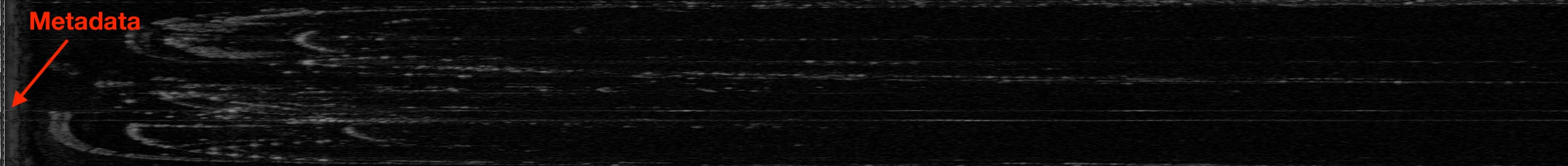
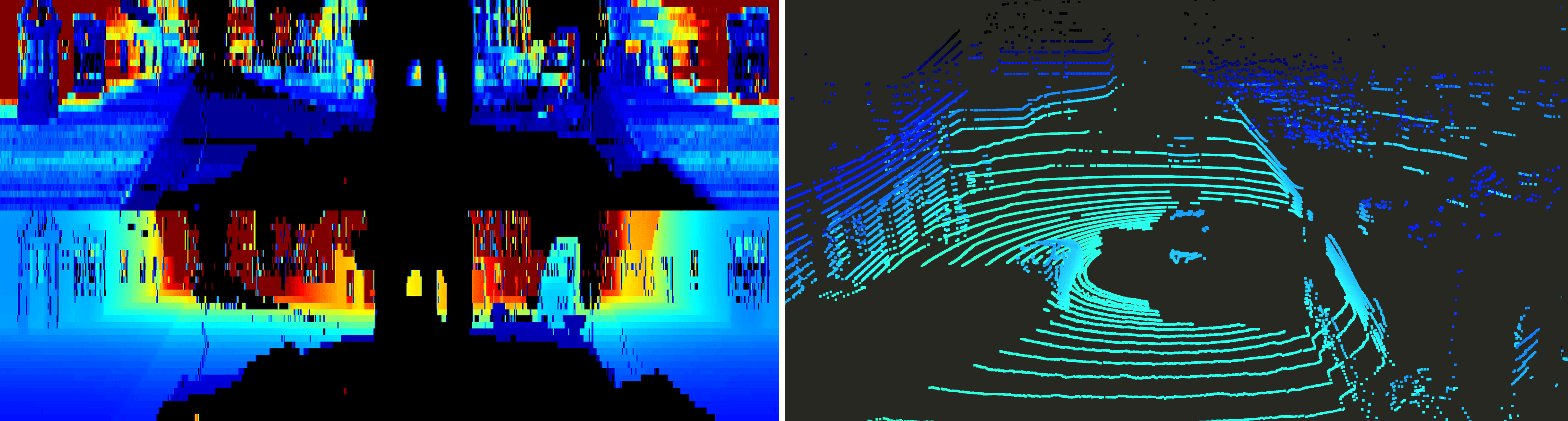
Velodyne Raw
Velodyne raw data is released as lossless PNG files with each column representing the sensor reading at each
azimuth. The files are structured as <laser>/<timestamp>.png, where <laser> is velodyne_left or velodyne_right
and <timestamp> is the UNIX timestamp of the capture, measured in microseconds. To give users all the raw data they
could need we also embed per azimuth metadata into the png into the following rows:
Intensities as uint8 in rows 1-32 - Raw intensity readings for each elevation.
Ranges Raw as uint16 in rows 33-96 - Raw range readings for each elevation, converted to metres with
ranges (metres) = ranges_raw * hdl32e_range_resolution where hdl32e_range_resolution = 0.02 m.
Sweep counter as uint16 in rows 97-98 - Converted to angle with azimuth (radians) = sweep_counter / encoder_size * 2 * pi
where encoder_size = 36000.
Approximate UNIX Timestamps as int64 in rows 99-106 - Timestamps are received for each data packet from the Velodyne LIDAR which includes 12 sets of readings for all 32 lasers. We have linearly interpolated timestamps at each azimuth reading but the user can extract the original received timestamps by simply taking every 12th timestamp.
The raw velodyne data can be converted into Cartesian (pointcloud) form using the development kit. Although approximately 2x slower than loading from the binary files, the raw files take approximately 8x less storage space.

Velodyne Binary
Velodyne binary data is released as single-precision floating point values packed into a binary file,
similar to the Velodyne scan format in the KITTI dataset. The files are structured
as <laser>/<timestamp>.bin, where <laser> is velodyne_left or velodyne_right and <timestamp> is the UNIX
timestamp of the capture, measured in microseconds.
Each scan consists of (x, y, z, I) x N values, where x, y, z are the 3D Cartesian coordinates of the LIDAR return relative to the sensor (in metres), and I is the measured intensity value.
No correction for the motion of the vehicle has been performed when projecting the points into Cartesian coordinates; this can be performed by modifying the function for projecting Velodyne Raw Data into Cartesian coordinates to account for motion using the supplied interpolated timestamps for each azimuth.
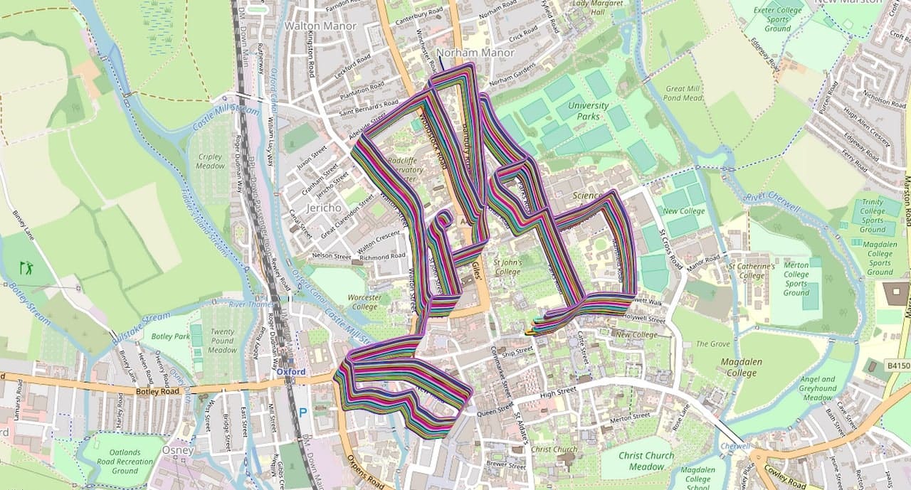
Ground Truth Radar Odometry
Alongside this dataset we provide ground truth SE2 radar odometry temporally aligned to the radar data (provided in an ASCII-formatted csv file). The poses were generated by performing a large-scale optimisation with Ceres Solver using robust visual odometry 2, visual loop closures 3 and GPS/INS as constraints. Further information can be found in the upcoming dataset paper.
The file radar_odometry.csv contains the SE(2) relative pose solution, consisting of the source and destination frame
UNIX timestamps (chosen to be in the middle of the corresponding radar scans), the six-vector Euler parameterisation
(x, y, z, α, β, γ) of the SE(3) relative pose relating the two frames (where z, α, β are all zero) and the starting
source and destination frame UNIX timestamps of the corresponding radar scans (which can be used to load the
corresponding radar data files).
Development Kit
The necessary functionality to load and parse the Radar and Velodyne data is provided in the original Oxford RobotCar Dataset Development Kit which can be downloaded on the downloads page. The same functions for 3D Pointcloud Generation and Pointcloud Projection Into Images as described in the original Oxford RobotCar Dataset Documentation can also be used with Velodyne data
Radar Loading and Conversion to Cartesian
For full demo usage please see PlayRadar.m and play_radar.py.
MATLAB:
The function LoadRadar reads raw radar data from a specified directory and at a specified timestamp, and returns
MATLAB format timestamps, azimuths, valid, fft_data and radar resolution as described in the sensor data above. The
function RadarPolarToCartesian can then take the polar radar data and convert it to Cartesian form as shown below.
Python:
The function radar.load_radar reads raw radar data from a specified directory and at a specified timestamp, and returns
MATLAB format timestamps, azimuths, valid, fft_data and radar resolution as described in the sensor data above. The
function radar.radar_polar_to_cartesian can then take the polar radar data and convert it to Cartesian form as shown below.
Velodyne Loading and Conversion to Pointcloud
For full demo usage please see PlayVelodyne.m and play_velodyne.py which can:
- Visualise the raw Velodyne data (intensities and ranges).
- Visualise the raw Velodyne data (intensities and ranges) interpolated to consistent azimuth angles between scans.
- Visualise the raw Velodyne data converted to a pointcloud (converts files of the form
<timestamp>.pngto pointcloud). - Visualise the binary Velodyne pointclouds (files of the form
<timestamp>.bin). This is approximately 2x faster than running the conversion from raw dataraw_ptcldat the cost of approximately 8x the storage space.
MATLAB
The function LoadVelodyneRaw reads raw Velodyne data from a specified directory and at a specified timestamp, and
returns MATLAB format ranges, intensities, angles, approximate_timestamps as described in the sensor data above. The
function VelodyneRawToPointcloud can then take the polar radar data and convert it to Cartesian
(pointcloud) form as shown below. The function LoadVelodyneBinary reads binary Velodyne data from a specified
directory and at a specified timestamp and returns the precomputed (x, y, z, intensity) pointcloud (not motion
compensated).
Python
The function velodyne.load_velodyne_raw reads raw Velodyne data from a specified directory and at a specified
timestamp, and returns MATLAB format ranges, intensities, angles, approximate_timestamps as described in the sensor data
above. The function velodyne.velodyne_raw_to_pointcloud can then take the polar radar data and
convert it to Cartesian (pointcloud) form as shown below. The function velodyne.load_velodyne_binary reads binary
Velodyne data from a specified directory and at a specified timestamp and returns the precomputed (x, y, z, intensity)
pointcloud (not motion compensated).
-
1 Year, 1000km: The Oxford RobotCar Dataset
Will Maddern and Geoff Pascoe and Chris Linegar and Paul Newman
The International Journal of Robotics Research 2017 ↩ -
Driven to Distraction: Self-Supervised Distractor Learning for Robust Monocular Visual Odometry in Urban Environments
Dan Barnes, Will Maddern, Ingmar Posner
International Conference on Robotics and Automation (ICRA) 2018 ↩ -
Appearance-only SLAM at Large Scale with FAB-MAP 2.0
M. Cummins and P. Newman
The International Journal of Robotics Research 2010 ↩